One question I keep coming back to in olfaction is deceptively simple: before odors reach the downstream classifier-like layers of the brain, what should the early circuit do to the raw receptor responses?
Olfactory receptor neurons (ORNs) already transform chemical mixtures into neural activity. But their responses can be redundant, correlated, and strongly shaped by nuisance variables such as total concentration. A good preprocessing circuit should keep the useful relationships between odors while making the representation more efficient for downstream computation.
This is where similarity matching becomes a useful lens.
The Basic Idea
Suppose we collect odor responses into a data matrix:
1 | X = [x(1), x(2), ..., x(T)] |
Each column is one odor sample, and each row is one neural channel. A similarity matching objective asks the output representation Y to preserve the pairwise geometry of the input:
1 | input similarity: X.T X |
In words: if two odors are similar in the input representation, they should remain similar in the output; if they are different, the output should keep them apart. That sounds almost too broad, but the power of the framework is that once we impose neural constraints, the objective can become a biologically plausible circuit.
Pehlevan, Sengupta, and Chklovskii showed that similarity matching objectives can lead to networks with local Hebbian and anti-Hebbian learning rules. The global geometry problem can be rewritten using auxiliary variables so that each synapse updates from local pre- and post-synaptic activity.
That is the beautiful move: a high-level coding principle turns into a mechanistic network.
From Similarity Matching to an Olfactory Circuit
In the olfactory preprocessing model I am studying, the circuit has three main activity variables:
1 | x(t): ORN input response to odor t |
The lateral population z is not just a nuisance variable. It represents the dominant features or directions that the circuit uses to reshape the output code. The recurrent and reciprocal interactions can be written schematically as:
with slow activity-dependent updates:
The exact constants matter for implementation, but the intuition is simpler:
Wlearns correlations between the output channels and lateral features.Mlearns correlations within the lateral population.- The lateral loop suppresses dominant shared structure in the ORN representation.
- The output becomes more spectrally balanced and less pairwise correlated.
This is the connection to the preprocessing circuit studied by Chapochnikov, Pehlevan, and Chklovskii. In that work, a similarity-matching-derived circuit provides a normative and mechanistic account of how olfactory representations can be normalized, partially whitened, and decorrelated.
Partial Whitening, Not Magic Whitening
One important point for my thesis is that this LC-style preprocessing is not the same thing as PCA whitening.
PCA whitening is an idealized operation: it rotates the data into principal components and rescales every dimension so the covariance becomes the identity matrix. That is useful as a reference, but it is not the literal computation of the biological circuit.
The LC model is more constrained. In the closed-form view, the circuit mainly shrinks the leading singular directions of the input. If the circuit has K lateral units, then K controls how many dominant directions can be directly acted on. The parameter rho changes the strength and shape of the spectral shrinkage, but increasing rho is not the same as turning the circuit into exact whitening.
So the right phrase is:
LC performs partial decorrelation or partial spectral equalization, not full PCA whitening.
That distinction matters. Otherwise it is too easy to overstate what the network is doing.
My Current Diagnostic Figure
The figure below compares three representations in my current synthetic olfactory setting: the ORN response, the LC-preprocessed response, and an idealized PCA-whitened reference.
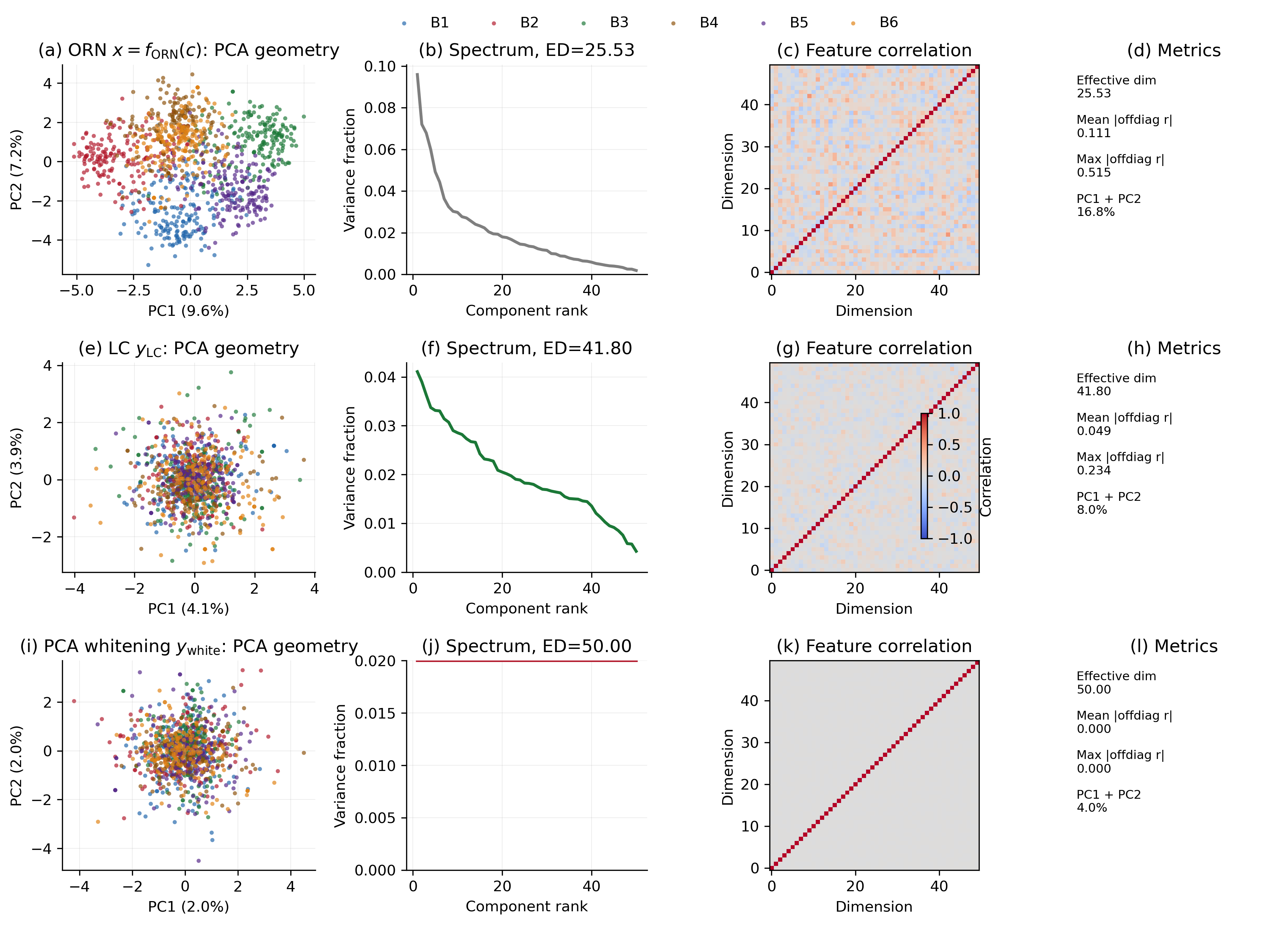
The main numbers are:
| Representation | Effective dimension | Mean abs offdiag r | Max abs offdiag r | PC1 + PC2 |
|---|---|---|---|---|
| ORN response | 25.53 | 0.111 | 0.515 | 16.8% |
| LC output | 41.80 | 0.049 | 0.234 | 8.0% |
| PCA whitening | 50.00 | 0.000 | 0.000 | 4.0% |
There are a few things I like about this diagnostic.
First, the ORN representation is no longer dominated by a trivial total-concentration axis. In an earlier dense sensitivity setup, nearly every ORN responded positively to nearly every molecule, so the first PC mostly measured “how much odor is present.” After composition normalization and sparse balanced receptor tuning, the ORN geometry is much healthier.
Second, the LC transformation clearly moves the representation toward a flatter, less redundant code. The effective dimension increases from 25.53 to 41.80, and the mean off-diagonal feature correlation falls from 0.111 to 0.049.
Third, PCA whitening is useful as a ceiling, not as the biological target. It reaches effective dimension 50 and zero off-diagonal correlations by construction. The LC output approaches that direction but remains a constrained circuit computation.
Why This Does Not Automatically Improve Classification
One subtle lesson from this project is that better decorrelation metrics do not guarantee better classification accuracy.
For the dominant molecular-block task, linear classifiers in the current setup are already strong on the ORN representation. The LC output slightly improves coding efficiency, but downstream accuracy depends on the label rule, noise, thresholds, and the random sparse expansion used by Kenyon-cell-like layers.
In my current runs, the rough picture is:
1 | without KC expansion: |
That is not a failure of the LC model. It is a warning about the task. A preprocessing circuit can be excellent at reducing redundancy and still not improve a particular supervised readout if the original representation already exposes the label structure.
For me, the interesting question is not simply “does LC increase accuracy?” It is:
1 | Under which odor statistics, noise regimes, and downstream constraints |
That question feels much closer to the biology.
What I Want to Understand Next
The next stage of this project is to study the network itself more deeply:
- how
Kcontrols the number of suppressed principal directions; - how
rhochanges the shrinkage curve without becoming exact whitening; - when partial decorrelation helps downstream sparse random expansion;
- how online learning adapts when the odor distribution shifts;
- whether the same circuit can be interpreted as both efficient coding and feature extraction.
Similarity matching is attractive because it does not stop at a descriptive statement like “the circuit decorrelates odors.” It gives a bridge from objective, to dynamics, to synaptic rules, to measurable representational geometry.
That bridge is the part I want to keep building.
References
- Chapochnikov, N., Pehlevan, C., and Chklovskii, D. B. (2023). Normative and mechanistic model of an adaptive circuit for efficient encoding and feature extraction.
- Pehlevan, C., Sengupta, A. M., and Chklovskii, D. B. (2018). Why Do Similarity Matching Objectives Lead to Hebbian/Anti-Hebbian Networks?. Also available on arXiv.